24 Epidemic modeling
24.1 Overview
There exists a growing body of tools for epidemic modelling that lets us conduct fairly complex analyses with minimal effort. This section will provide an overview on how to use these tools to:
- estimate the effective reproduction number Rt and related statistics such as the doubling time
- produce short-term projections of future incidence
It is not intended as an overview of the methodologies and statistical methods underlying these tools, so please refer to the Resources tab for links to some papers covering this. Make sure you have an understanding of the methods before using these tools; this will ensure you can accurately interpret their results.
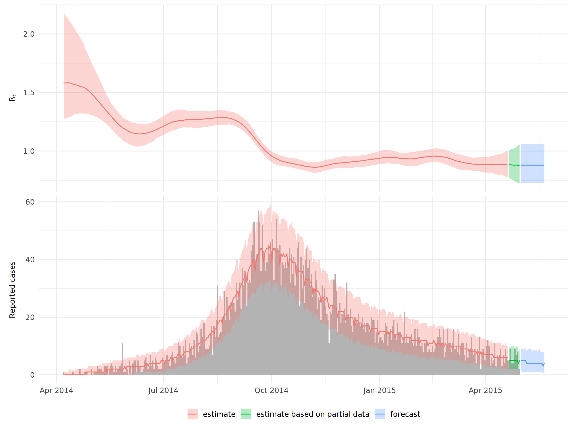
Below is an example of one of the outputs we’ll be producing in this section.
24.2 Preparation
We will use two different methods and packages for Rt estimation, namely EpiNow and EpiEstim, as well as the projections package for forecasting case incidence.
This code chunk shows the loading of packages required for the analyses. In this handbook we emphasize p_load() from pacman, which installs the package if necessary and loads it for use. You can also load installed packages with library() from base R. See the page on R basics for more information on R packages.
pacman::p_load(
   rio,          # File import
   here,         # File locator
   tidyverse,    # Data management + ggplot2 graphics
   epicontacts,  # Analysing transmission networks
   EpiNow2,      # Rt estimation
   EpiEstim,     # Rt estimation
   projections,  # Incidence projections
   incidence2,   # Handling incidence data
   incidence,    # Incidence objects for projections
   epitrix,      # Useful epi functions
   distcrete     # Discrete delay distributions
)
We will use the cleaned case linelist for all analyses in this section. If you want to follow along, click to download the “clean” linelist (as .rds file). See the Download handbook and data page to download all example data used in this handbook.
# import the cleaned linelist
linelist <- import("linelist_cleaned.rds")
24.3 Estimating Rt
EpiNow2 vs. EpiEstim
The reproduction number R is a measure of the transmissibility of a disease and is defined as the expected number of secondary cases per infected case. In a fully susceptible population, this value represents the basic reproduction number R0. However, as the number of susceptible individuals in a population changes over the course of an outbreak or pandemic, and as various response measures are implemented, the most commonly used measure of transmissibility is the effective reproduction number Rt; this is defined as the expected number of secondary cases per infected case at a given time t.
The EpiNow2 package provides the most sophisticated framework for estimating Rt. It has two key advantages over the other commonly used package, EpiEstim:
- It accounts for delays in reporting and can therefore estimate Rt even when recent data is incomplete.
- It estimates Rt on dates of infection rather than the dates of onset of reporting, which means that the effect of an intervention will be immediately reflected in a change in Rt, rather than with a delay.
However, it also has two key disadvantages:
- It requires knowledge of the generation time distribution (i.e. distribution of delays between infection of a primary and secondary cases), incubation period distribution (i.e. distribution of delays between infection and symptom onset) and any further delay distribution relevant to your data (e.g. if you have dates of reporting, you require the distribution of delays from symptom onset to reporting). While this will allow more accurate estimation of Rt, EpiEstim only requires the serial interval distribution (i.e. the distribution of delays between symptom onset of a primary and a secondary case), which may be the only distribution available to you.
- EpiNow2 is significantly slower than EpiEstim, anecdotally by a factor of about 100-1000! For example, estimating Rt for the sample outbreak considered in this section takes about four hours (this was run for a large number of iterations to ensure high accuracy and could probably be reduced if necessary, however the points stands that the algorithm is slow in general). This may be unfeasible if you are regularly updating your Rt estimates.
Which package you choose to use will therefore depend on the data, time and computational resources available to you.
EpiNow2
Estimating delay distributions
The delay distributions required to run EpiNow2 depend on the data you have. Essentially, you need to be able to describe the delay from the date of infection to the date of the event you want to use to estimate Rt. If you are using dates of onset, this would simply be the incubation period distribution. If you are using dates of reporting, you require the delay from infection to reporting. As this distribution is unlikely to be known directly, EpiNow2 lets you chain multiple delay distributions together; in this case, the delay from infection to symptom onset (e.g. the incubation period, which is likely known) and from symptom onset to reporting (which you can often estimate from the data).
As we have the dates of onset for all our cases in the example linelist, we will only require the incubation period distribution to link our data (e.g. dates of symptom onset) to the date of infection. We can either estimate this distribution from the data or use values from the literature.
A literature estimate of the incubation period of Ebola (taken from this paper) with a mean of 9.1, standard deviation of 7.3 and maximum value of 30 would be specified as follows:
incubation_period_lit <- LogNormal(
  mean = 9.1,
  sd = 7.3,
  max = 30
)
LogNormal() takes the mean and the standard deviation in days, on the natural scale, and converts them to the log scale itself. The max parameter cuts the distribution at 30 days.
In this analysis, we instead estimate the incubation period distribution from the linelist itself using the function bootstrapped_dist_fit, which will fit a lognormal distribution to the observed delays between infection and onset in the linelist.
## estimate incubation period
incubation_period <- bootstrapped_dist_fit(
  linelist$date_onset - linelist$date_infection,
  dist = "lognormal",
  max_value = 100,
  bootstraps = 1
)
The other distribution we require is the generation time. As we have data on infection times and transmission links, we can estimate this distribution from the linelist by calculating the delay between infection times of infector-infectee pairs. To do this, we use the handy get_pairwise function from the package epicontacts, which allows us to calculate pairwise differences of linelist properties between transmission pairs. We first create an epicontacts object (see Transmission chains page for further details):
## generate contacts
contacts <- linelist %>%
  transmute(
    from = infector,
    to = case_id
  ) %>%
  drop_na()

## generate epicontacts object
epic <- make_epicontacts(
  linelist = linelist,
  contacts = contacts,
  directed = TRUE
)
We then fit the difference in infection times between transmission pairs, calculated using get_pairwise, to a gamma distribution:
## estimate gamma generation time
generation_time <- bootstrapped_dist_fit(
  get_pairwise(epic, "date_infection"),
  dist = "gamma",
  max_value = 20,
  bootstraps = 1
)
Running EpiNow2
Now we just need to calculate daily incidence from the linelist, which we can do easily with the dplyr functions group_by() and n(). Note that EpiNow2 requires the column names to be date and confirm. EpiNow2 also stops with an error on a missing date, so we drop the cases without a date of onset. With gaps between the dates, EpiNow2 1.9.0 stopped with an error on these data. So fill_missing() adds the days without cases, with a count of 0.
## get incidence from onset dates
cases <- linelist %>%
  filter(!is.na(date_onset)) %>%
  group_by(date = date_onset) %>%
  summarise(confirm = n()) %>%
  ## add the days without cases, with a count of 0
  fill_missing(missing_dates = "zero")
We can then estimate Rt using the epinow function. Some notes on the inputs:
- The
generation_timeargument takes the generation time distribution inside thegt_optsfunction. - We can provide any number of ‘chained’ delay distributions to the
delaysargument. We would simply add them to theincubation_periodobject with+within thedelay_optsfunction. -
horizonin theforecast_optsfunction indicates how many days we want to project future incidence for. - We pass additional options to the
stanargument to specify how long we want to run the inference for. Increasingsamplesandchainswill give you a more accurate estimate that better characterises uncertainty, however will take longer to run.
## run epinow
epinow_res <- epinow(
  data = cases,
  generation_time = gt_opts(generation_time),
  delays = delay_opts(incubation_period),
  forecast = forecast_opts(horizon = 21),
  stan = stan_opts(samples = 750, chains = 4)
)
Analysing outputs
This page does not run the fit. The results below come from a fit that is stored in the appliedepidata package. An earlier version of EpiNow2 made that fit. The code above is the way to make such a fit with EpiNow2 1.9.
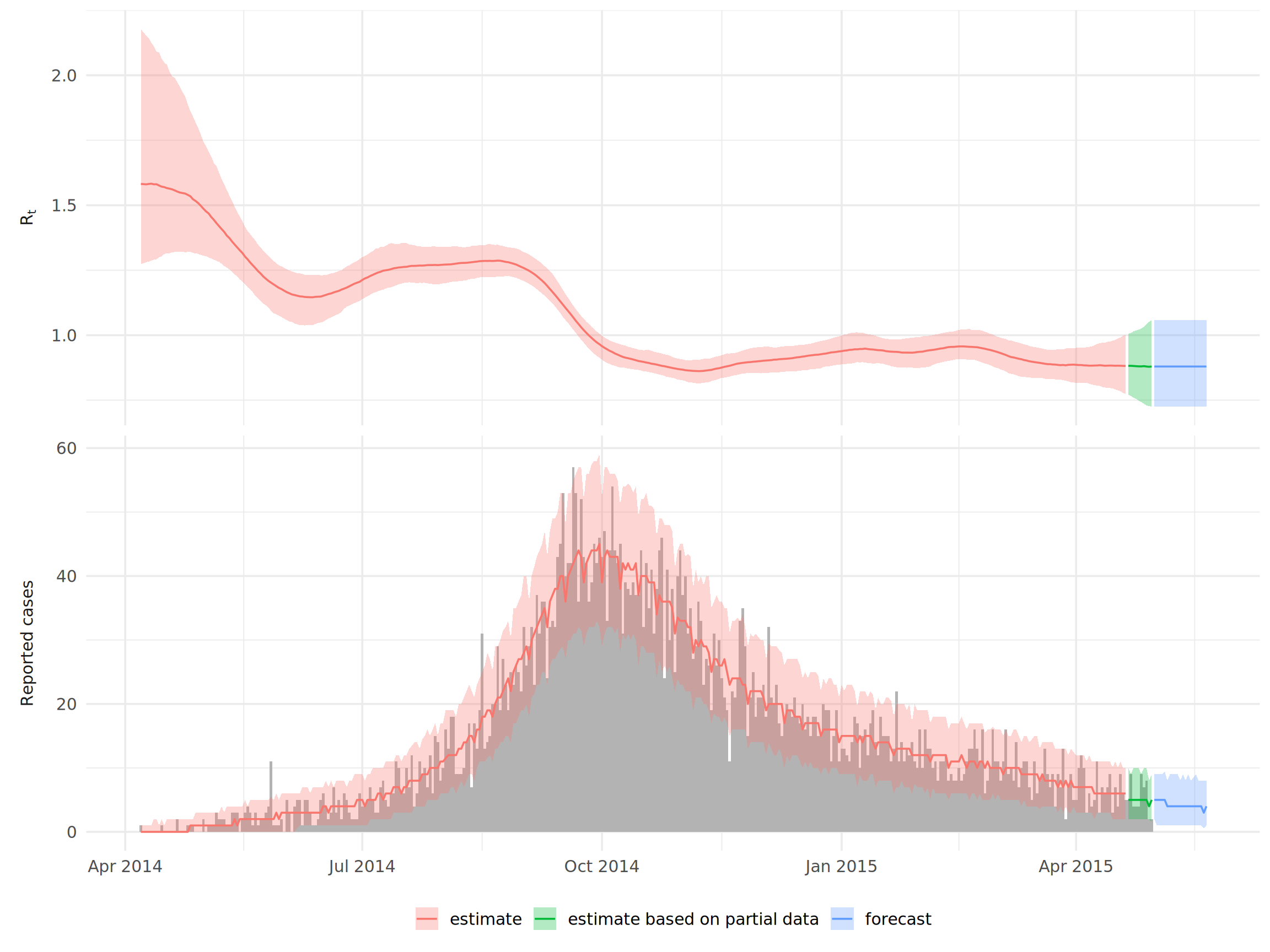
On a fit from EpiNow2 1.9, the plot() function draws a summary figure, and the summary() function gives a summary table. These functions stop with an error on the stored fit. So we load the tables of the stored fit and plot them with ggplot2:
## load the stored estimates and the case counts that the fit used
estimates <- appliedepidata::get_data(name = "epidemic_models_summarised_estimates")
observations <- appliedepidata::get_data(name = "epidemic_models_reported_cases")

## plot summary figure
ggplot(
  data = filter(estimates, variable %in% c("R", "reported_cases")),
  aes(x = date)
) +
  ## observed case counts, in the reported cases panel only
  geom_col(
    data = mutate(observations, variable = "reported_cases"),
    aes(y = confirm),
    fill = "grey70",
    width = 1
  ) +
  ## 90% credible interval and median, coloured by estimate type
  geom_ribbon(aes(ymin = lower_90, ymax = upper_90, fill = type), alpha = 0.3) +
  geom_line(aes(y = median, colour = type)) +
  ## use label_parsed to allow subscript label
  facet_wrap(
    ~ variable,
    ncol = 1,
    scales = "free_y",
    labeller = as_labeller(c("R" = "R[t]", "reported_cases" = "Reported~cases"), label_parsed),
    strip.position = 'left'
  ) +
  labs(x = NULL, y = NULL, colour = NULL, fill = NULL) +
  theme_minimal(base_size = 14) +
  theme(
    strip.background = element_blank(),
    strip.placement = 'outside',
    legend.position = 'bottom'
  )
We can also look at various summary statistics:
## summary table of the stored fit
summary_table <- appliedepidata::get_data(name = "epidemic_models_summary")
summary_table[, c("measure", "estimate")]
measure estimate
1 New confirmed cases by infection date 4 (2 -- 6)
2 Expected change in daily cases Unsure
3 Effective reproduction no. 0.88 (0.73 -- 1.1)
4 Rate of growth -0.012 (-0.028 -- 0.0052)
5 Doubling/halving time (days) -60 (130 -- -25)For further analyses and custom plotting, you can access the summarised daily estimates of a fit from EpiNow2 1.9 with summary(epinow_res, type = "parameters"). We will convert this from the default data.table to a tibble for ease of use with dplyr. The table below shows the same estimates from the stored fit.
## extract summary and convert to tibble
estimates <- as_tibble(summary(epinow_res, type = "parameters"))
estimates
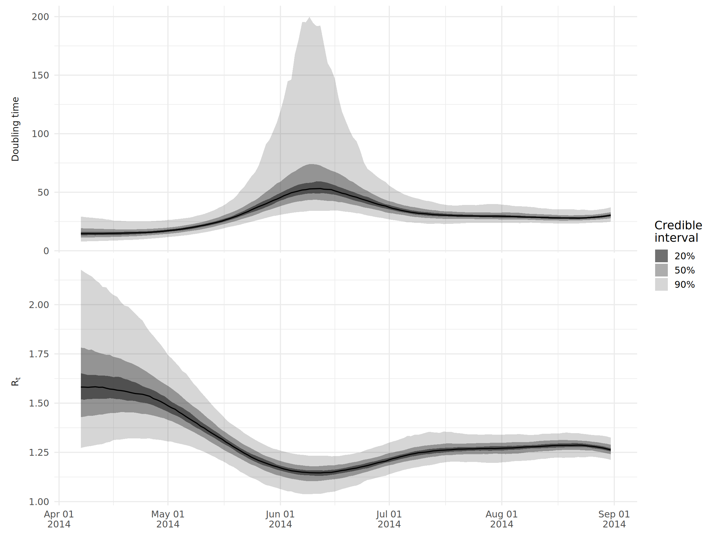
As an example, let’s make a plot of the doubling time and Rt. We will only look at the first few months of the outbreak when Rt is well above one, to avoid plotting extremely high doublings times.
We use the formula log(2)/growth_rate to calculate the doubling time from the estimated growth rate.
## make wide df for median plotting
df_wide <- estimates %>%
  filter(
    variable %in% c("growth_rate", "R"),
    date < as.Date("2014-09-01")
  ) %>%
  ## convert growth rates to doubling times
  mutate(
    across(
      c(median, lower_90:upper_90),
      ~ case_when(
        variable == "growth_rate" ~ log(2)/.x,
        TRUE ~ .x
      )
    ),
    ## rename variable to reflect transformation
    variable = replace(variable, variable == "growth_rate", "doubling_time")
  )

## make long df for quantile plotting
df_long <- df_wide %>%
  ## here we match matching quantiles (e.g. lower_90 to upper_90)
  pivot_longer(
    lower_90:upper_90,
    names_to = c(".value", "quantile"),
    names_pattern = "(.+)_(.+)"
  )

## make plot
ggplot() +
  geom_ribbon(
    data = df_long,
    aes(x = date, ymin = lower, ymax = upper, alpha = quantile),
    color = NA
  ) +
  geom_line(
    data = df_wide,
    aes(x = date, y = median)
  ) +
  ## use label_parsed to allow subscript label
  facet_wrap(
    ~ variable,
    ncol = 1,
    scales = "free_y",
    labeller = as_labeller(c(R = "R[t]", doubling_time = "Doubling~time"), label_parsed),
    strip.position = 'left'
  ) +
  ## manually define quantile transparency
  scale_alpha_manual(
    values = c(`20` = 0.7, `50` = 0.4, `90` = 0.2),
    labels = function(x) paste0(x, "%")
  ) +
  labs(
    x = NULL,
    y = NULL,
    alpha = "Credible\ninterval"
  ) +
  scale_x_date(
    date_breaks = "1 month",
    date_labels = "%b %d\n%Y"
  ) +
  theme_minimal(base_size = 14) +
  theme(
    strip.background = element_blank(),
    strip.placement = 'outside'
  )
EpiEstim
To run EpiEstim, we need to provide data on daily incidence and specify the serial interval (i.e. the distribution of delays between symptom onset of primary and secondary cases).
Incidence data can be provided to EpiEstim as a vector, a data frame, or an incidence object from the original incidence package. You can even distinguish between imports and locally acquired infections; see the documentation at ?estimate_R for further details.
We will create the input using incidence2. See the page on Epidemic curves for more examples with the incidence2 package. Since there have been updates to the incidence2 package that don’t completely align with estimate_R()’s expected input, there are some minor additional steps needed. The incidence object consists of a tibble with dates and their respective case counts. We use complete() from tidyr to ensure all dates are included (even those with no cases), and then rename() the columns to align with what is expected by estimate_R() in a later step.
## get incidence from onset date
cases <- incidence2::incidence(linelist, date_index = "date_onset") %>% # get case counts by day
  tidyr::complete(date_index = seq.Date(                              # ensure all dates are represented
    from = min(date_index, na.rm = T),
    to = max(date_index, na.rm=T),
    by = "day"),
    fill = list(count = 0)) %>%                                       # convert NA counts to 0
  rename(I = count,                                                   # rename to names expected by estimate_R()
         dates = date_index)
The package provides several options for specifying the serial interval, the details of which are provided in the documentation at ?estimate_R. We will cover two of them here.
Using serial interval estimates from the literature
Using the option method = "parametric_si", we can manually specify the mean and standard deviation of the serial interval in a config object created using the function make_config. We use a mean and standard deviation of 12.0 and 5.2, respectively, defined in this paper.
By default, estimate_R() uses weekly sliding windows from the second day of the data. EpiEstim warns that Rt estimated from very few cases is unreliable: with its default settings, it needs at least 11 cases in a window. The first weeks of this outbreak hold fewer. So we start the weekly windows at the first 7-day window that holds at least 11 cases. Both runs below use these windows:
## daily case counts, one row per day
daily_cases <- cases$I

## number of cases in the 7-day window that starts on each day
window_cases <- sapply(
  seq_len(length(daily_cases) - 6),
  function(t) sum(daily_cases[t:(t + 6)])
)

## weekly sliding windows from the first window with at least 11 cases
weekly_start <- max(2, which(window_cases >= 11)[1]):(length(daily_cases) - 6)
weekly_end <- weekly_start + 6

## make config
config_lit <- make_config(
  mean_si = 12.0,
  std_si = 5.2,
  t_start = weekly_start,
  t_end = weekly_end
)
We can then estimate Rt with the estimate_R function:
cases <- cases %>%
     filter(!is.na(dates))


#create a dataframe for the function estimate_R()
cases_incidence <- data.frame(dates = seq.Date(from = min(cases$dates),
                               to = max(cases$dates),
                               by = 1))

cases_incidence <- left_join(cases_incidence, cases, by = "dates") %>%
     select(dates, I) %>%
     mutate(I = ifelse(is.na(I), 0, I))

epiestim_res_lit <- estimate_R(
  incid = cases_incidence,
  method = "parametric_si",
  config = config_lit
)
and plot the Rt estimates. The plot() function of EpiEstim raises a deprecation warning from ggplot2, so we write a short function that plots the estimates with ggplot2. It dates each estimate by the end of its time window:
## plot the mean R estimate and its 95% credible interval
plot_rt <- function(res) {
  res$R %>%
    ## drop the time windows without an estimate
    filter(!is.na(`Mean(R)`)) %>%
    ## date each estimate by the end of its time window
    mutate(date = res$dates[t_end]) %>%
    ggplot(aes(x = date)) +
    geom_ribbon(aes(ymin = `Quantile.0.025(R)`, ymax = `Quantile.0.975(R)`), alpha = 0.3) +
    geom_line(aes(y = `Mean(R)`)) +
    geom_hline(yintercept = 1, linetype = 2) +
    labs(x = NULL, y = expression(R[t])) +
    theme_minimal(base_size = 14)
}

plot_rt(epiestim_res_lit)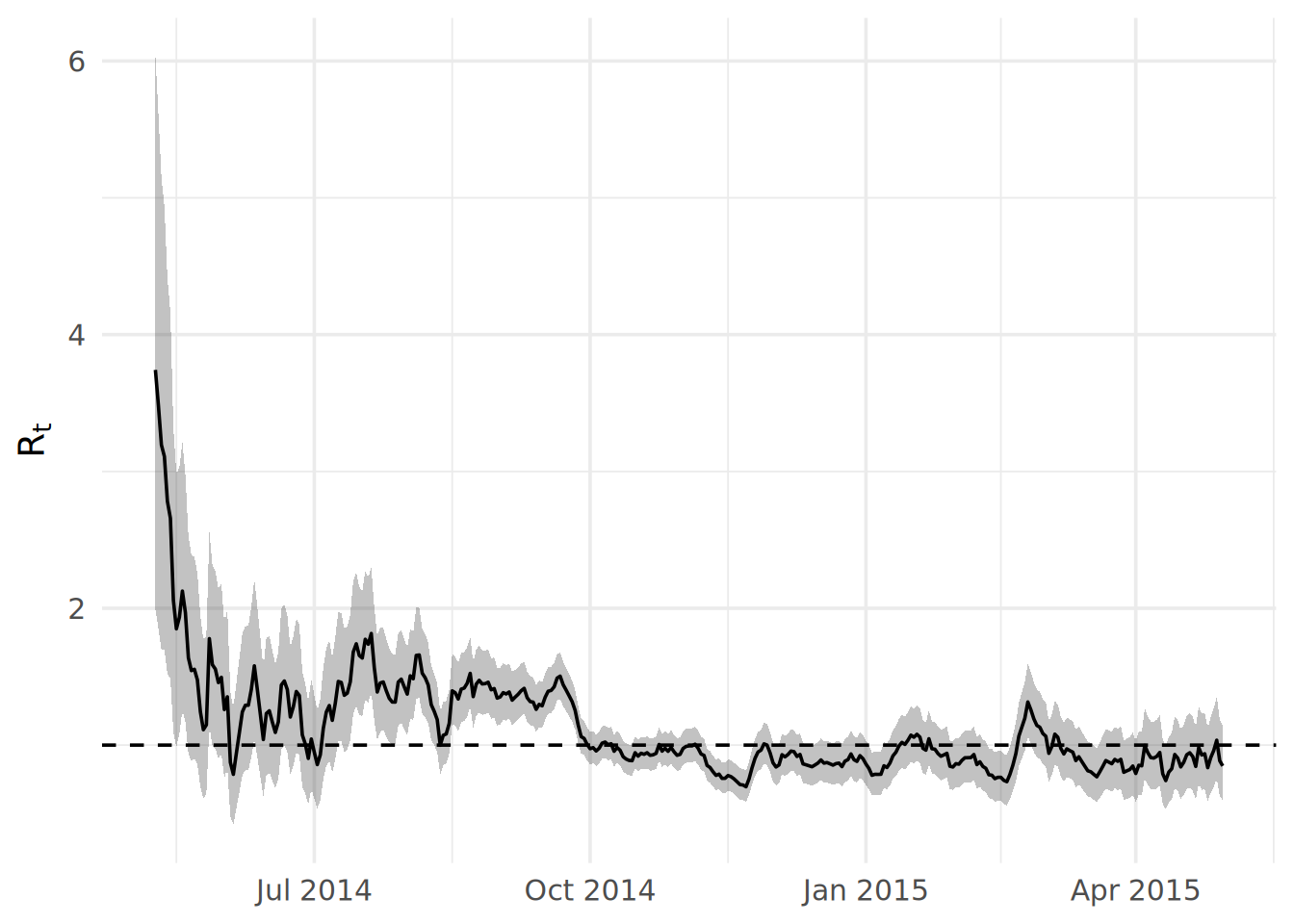
Using serial interval estimates from the data
As we have data on dates of symptom onset and transmission links, we can also estimate the serial interval from the linelist by calculating the delay between onset dates of infector-infectee pairs. As we did in the EpiNow2 section, we will use the get_pairwise function from the epicontacts package, which allows us to calculate pairwise differences of linelist properties between transmission pairs. We first create an epicontacts object (see Transmission chains page for further details):
## generate contacts
contacts <- linelist %>%
  transmute(
    from = infector,
    to = case_id
  ) %>%
  drop_na()

## generate epicontacts object
epic <- make_epicontacts(
  linelist = linelist,
  contacts = contacts,
  directed = TRUE
)
We then fit the difference in onset dates between transmission pairs, calculated using get_pairwise, to a gamma distribution. We use the handy fit_disc_gamma from the epitrix package for this fitting procedure, as we require a discretised distribution.
## estimate gamma serial interval, without the pairs that have no onset date
serial_interval <- fit_disc_gamma(na.omit(get_pairwise(epic, "date_onset")))
We then pass this information to the config object, run EpiEstim again and plot the results:
## make config
config_emp <- make_config(
  mean_si = serial_interval$mu,
  std_si = serial_interval$sd,
  t_start = weekly_start,
  t_end = weekly_end
)

## run epiestim
epiestim_res_emp <- estimate_R(
  incid = cases_incidence,
  method = "parametric_si",
  config = config_emp
)

## plot outputs
plot_rt(epiestim_res_emp)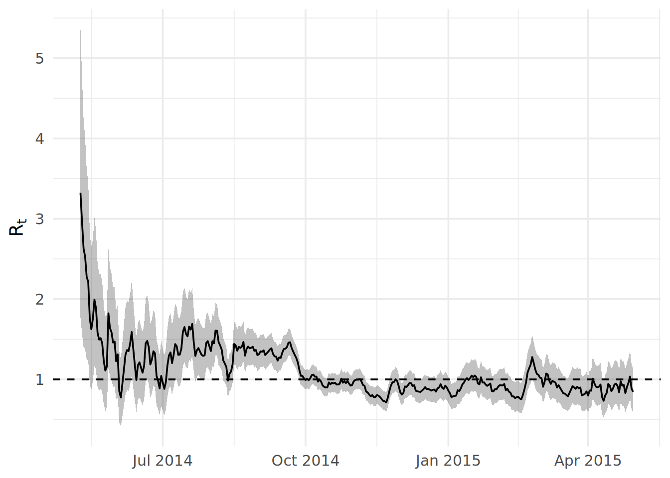
Specifying estimation time windows
You can also choose the start of the windows yourself, for example to estimate Rt only from 1 June 2014, as shown below. Unfortunately, EpiEstim only provides a very clunky way of specifying these estimations times, in that you have to provide a vector of integers referring to the start and end dates for each time window.
## define a vector of dates starting on June 1st
start_dates <- seq.Date(
  as.Date("2014-06-01"),
  max(cases$dates) - 7,
  by = 1
) %>%
  ## subtract the starting date to convert to numeric
  `-`(min(cases$dates)) %>%
  ## convert to integer
  as.integer() %>%
  ## add 1, because day 1 of the incidence data is its first date
  `+`(1L)

## add six days for a one week sliding window
end_dates <- start_dates + 6

## make config
config_partial <- make_config(
  mean_si = 12.0,
  std_si = 5.2,
  t_start = start_dates,
  t_end = end_dates
)
Now we re-run EpiEstim and can see that the estimates only start from June:
## run epiestim
epiestim_res_partial <- estimate_R(
  incid = cases_incidence,
  method = "parametric_si",
  config = config_partial
)

## plot outputs
plot_rt(epiestim_res_partial)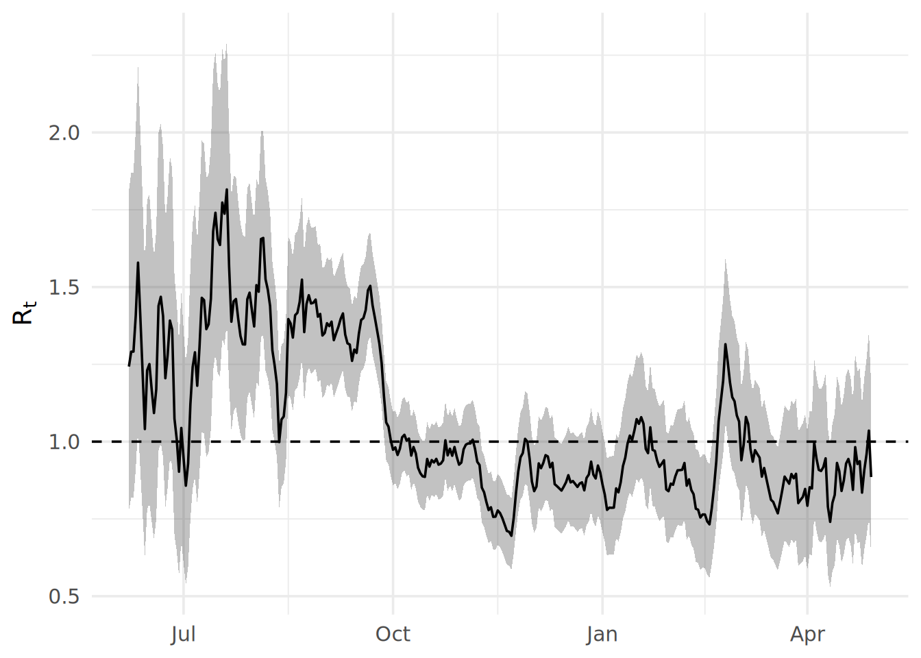
Analysing outputs
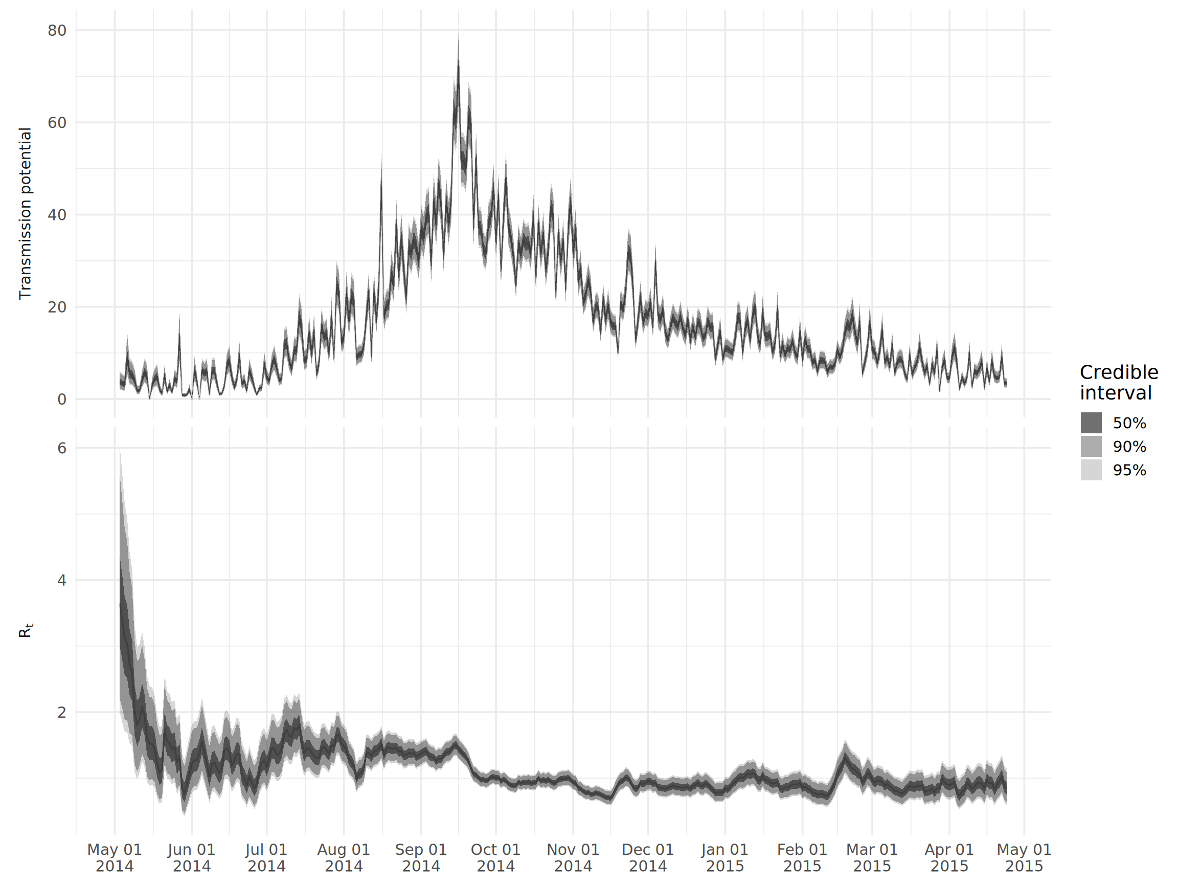
The main outputs can be accessed via $R. As an example, we will create a plot of Rt and a measure of “transmission potential” given by the product of Rt and the number of cases reported on that day; this represents the expected number of cases in the next generation of infection.
## make wide dataframe for median
df_wide <- epiestim_res_lit$R %>%
  rename_all(clean_labels) %>%
  rename(
    lower_95_r = quantile_0_025_r,
    lower_90_r = quantile_0_05_r,
    lower_50_r = quantile_0_25_r,
    upper_50_r = quantile_0_75_r,
    upper_90_r = quantile_0_95_r,
    upper_95_r = quantile_0_975_r,
    ) %>%
  ## drop the time windows without an estimate
  filter(!is.na(mean_r)) %>%
  mutate(
    ## extract the median date from t_start and t_end
    dates = epiestim_res_emp$dates[round(map2_dbl(t_start, t_end, median))],
    var = "R[t]"
  ) %>%
  ## merge in daily incidence data
  left_join(cases, "dates") %>%
  ## calculate risk across all r estimates
  mutate(
    across(
      lower_95_r:upper_95_r,
      ~ .x*I,
      .names = "{str_replace(.col, '_r', '_risk')}"
    )
  ) %>%
  ## seperate r estimates and risk estimates
  pivot_longer(
    contains("median"),
    names_to = c(".value", "variable"),
    names_pattern = "(.+)_(.+)"
  ) %>%
  ## assign factor levels
  mutate(variable = factor(variable, c("risk", "r")))

## make long dataframe from quantiles
df_long <- df_wide %>%
  select(-variable, -median) %>%
  ## seperate r/risk estimates and quantile levels
  pivot_longer(
    contains(c("lower", "upper")),
    names_to = c(".value", "quantile", "variable"),
    names_pattern = "(.+)_(.+)_(.+)"
  ) %>%
  mutate(variable = factor(variable, c("risk", "r")))

## make plot
ggplot() +
  geom_ribbon(
    data = df_long,
    aes(x = dates, ymin = lower, ymax = upper, alpha = quantile),
    color = NA
  ) +
  geom_line(
    data = df_wide,
    aes(x = dates, y = median),
    alpha = 0.2
  ) +
  ## use label_parsed to allow subscript label
  facet_wrap(
    ~ variable,
    ncol = 1,
    scales = "free_y",
    labeller = as_labeller(c(r = "R[t]", risk = "Transmission~potential"), label_parsed),
    strip.position = 'left'
  ) +
  ## manually define quantile transparency
  scale_alpha_manual(
    values = c(`50` = 0.7, `90` = 0.4, `95` = 0.2),
    labels = function(x) paste0(x, "%")
  ) +
  labs(
    x = NULL,
    y = NULL,
    alpha = "Credible\ninterval"
  ) +
  scale_x_date(
    date_breaks = "1 month",
    date_labels = "%b %d\n%Y"
  ) +
  theme_minimal(base_size = 14) +
  theme(
    strip.background = element_blank(),
    strip.placement = 'outside'
  )
24.4 Projecting incidence
EpiNow2
Besides estimating Rt, EpiNow2 also supports forecasting of Rt and projections of case numbers. All you need to do is give forecast_opts(horizon = 21) to the forecast argument of your epinow function call. The horizon is the number of days you want to project into the future. See the EpiNow2 section under the “Estimating Rt” for details on how to get EpiNow2 up and running. In this section, we will just plot the forecast from the stored fit.
## define minimum date for plot
min_date <- as.Date("2015-03-01")

## load the summarised estimates of the stored fit
estimates <- as_tibble(appliedepidata::get_data(name = "epidemic_models_summarised_estimates"))

## load the case counts that the stored fit used
observations <- as_tibble(appliedepidata::get_data(name = "epidemic_models_reported_cases")) %>%
  filter(date > min_date)

## extract forecasted estimates of case numbers
df_wide <- estimates %>%
  filter(
    variable == "reported_cases",
    type == "forecast",
    date > min_date
  )

## convert to even longer format for quantile plotting
df_long <- df_wide %>%
  ## here we match matching quantiles (e.g. lower_90 to upper_90)
  pivot_longer(
    lower_90:upper_90,
    names_to = c(".value", "quantile"),
    names_pattern = "(.+)_(.+)"
  )

## make plot
ggplot() +
  geom_col(
    data = observations,
    aes(x = date, y = confirm),
    width = 1
  ) +
  geom_ribbon(
    data = df_long,
    aes(x = date, ymin = lower, ymax = upper, alpha = quantile),
    color = NA
  ) +
  geom_line(
    data = df_wide,
    aes(x = date, y = median)
  ) +
  geom_vline(xintercept = min(df_long$date), linetype = 2) +
  ## manually define quantile transparency
  scale_alpha_manual(
    values = c(`20` = 0.7, `50` = 0.4, `90` = 0.2),
    labels = function(x) paste0(x, "%")
  ) +
  labs(
    x = NULL,
    y = "Daily reported cases",
    alpha = "Credible\ninterval"
  ) +
  scale_x_date(
    date_breaks = "1 month",
    date_labels = "%b %d\n%Y"
  ) +
  theme_minimal(base_size = 14)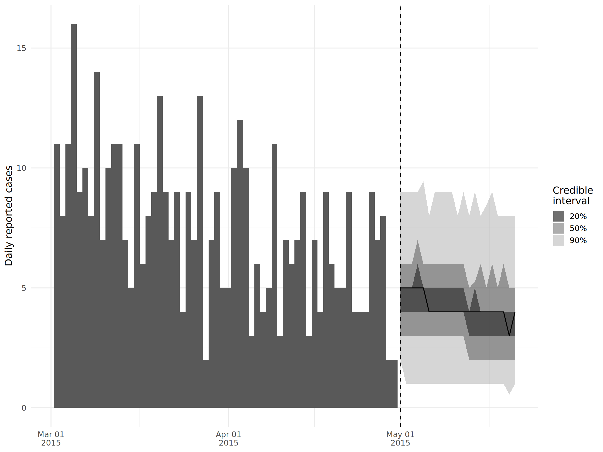
projections
The projections package developed by RECON makes it very easy to make short term incidence forecasts, requiring only knowledge of the effective reproduction number Rt and the serial interval. Here we will cover how to use serial interval estimates from the literature and how to use our own estimates from the linelist.
Using serial interval estimates from the literature
projections requires a discretised serial interval distribution of the class distcrete from the package distcrete. We will use a gamma distribution with a mean of 12.0 and and standard deviation of 5.2 defined in this paper. To convert these values into the shape and scale parameters required for a gamma distribution, we will use the function gamma_mucv2shapescale from the epitrix package.
## get shape and scale parameters from the mean mu and the coefficient of
## variation (e.g. the ratio of the standard deviation to the mean)
shapescale <- epitrix::gamma_mucv2shapescale(mu = 12.0, cv = 5.2/12)

## make distcrete object
serial_interval_lit <- distcrete::distcrete(
  name = "gamma",
  interval = 1,
  shape = shapescale$shape,
  scale = shapescale$scale
)
Here is a quick check to make sure the serial interval looks correct. We access the density of the gamma distribution we have just defined by $d, which is equivalent to calling dgamma:
## check to make sure the serial interval looks correct
ggplot(
  data = tibble(x = 0:50, y = serial_interval_lit$d(0:50)),
  aes(x = x, y = y)
) +
  geom_area() +
  labs(x = "Serial interval", y = "Density")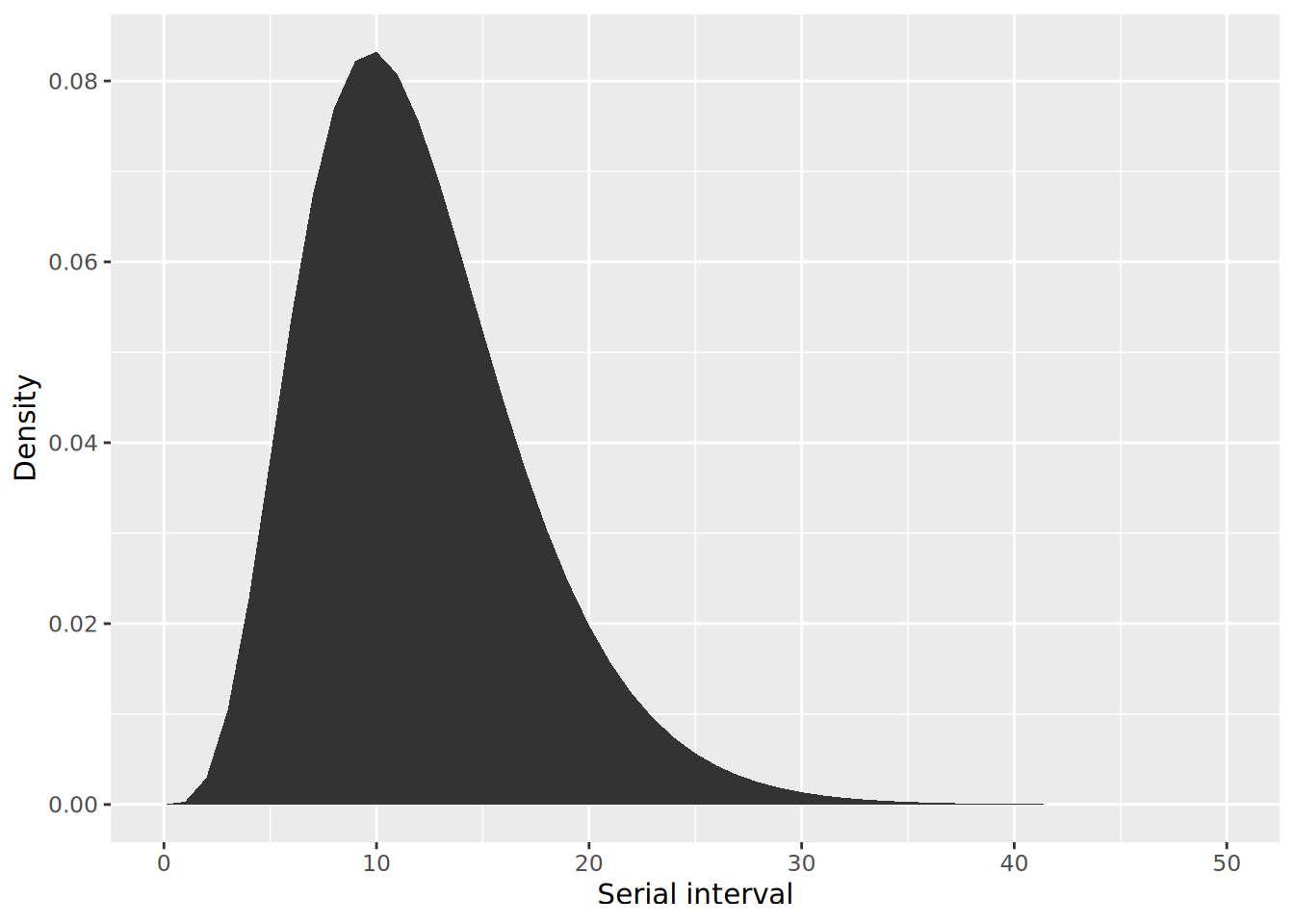
Using serial interval estimates from the data
As we have data on dates of symptom onset and transmission links, we can also estimate the serial interval from the linelist by calculating the delay between onset dates of infector-infectee pairs. As we did in the EpiNow2 section, we will use the get_pairwise function from the epicontacts package, which allows us to calculate pairwise differences of linelist properties between transmission pairs. We first create an epicontacts object (see Transmission chains page for further details):
## generate contacts
contacts <- linelist %>%
  transmute(
    from = infector,
    to = case_id
  ) %>%
  drop_na()

## generate epicontacts object
epic <- make_epicontacts(
  linelist = linelist,
  contacts = contacts,
  directed = TRUE
)
We then fit the difference in onset dates between transmission pairs, calculated using get_pairwise, to a gamma distribution. We use the handy fit_disc_gamma from the epitrix package for this fitting procedure, as we require a discretised distribution.
## estimate gamma serial interval, without the pairs that have no onset date
serial_interval <- fit_disc_gamma(na.omit(get_pairwise(epic, "date_onset")))

## inspect estimate
serial_interval[c("mu", "sd")]
$mu
[1] 11.51047
$sd
[1] 7.696056Projecting incidence
To project future incidence, we still need to provide historical incidence in the form of an incidence object, as well as a sample of plausible Rt values. We will generate these values using the Rt estimates generated by EpiEstim in the previous section (under “Estimating Rt”) and stored in the epiestim_res_emp object. In the code below, we extract the mean and standard deviation estimates of Rt for the last time window of the outbreak (using the tail function to access the last element in a vector), and simulate 1000 values from a gamma distribution using rgamma. You can also provide your own vector of Rt values that you want to use for forward projections.
## create incidence object from dates of onset, without the cases that have no onset date
inc <- incidence::incidence(na.omit(linelist$date_onset))

## extract plausible r values from most recent estimate
mean_r <- tail(epiestim_res_emp$R$`Mean(R)`, 1)
sd_r <- tail(epiestim_res_emp$R$`Std(R)`, 1)
shapescale <- gamma_mucv2shapescale(mu = mean_r, cv = sd_r/mean_r)
plausible_r <- rgamma(1000, shape = shapescale$shape, scale = shapescale$scale)

## check distribution
ggplot(data = tibble(r = plausible_r), aes(x = r)) +
  geom_histogram(bins = 30) +
  labs(x = expression(R[t]), y = "Counts")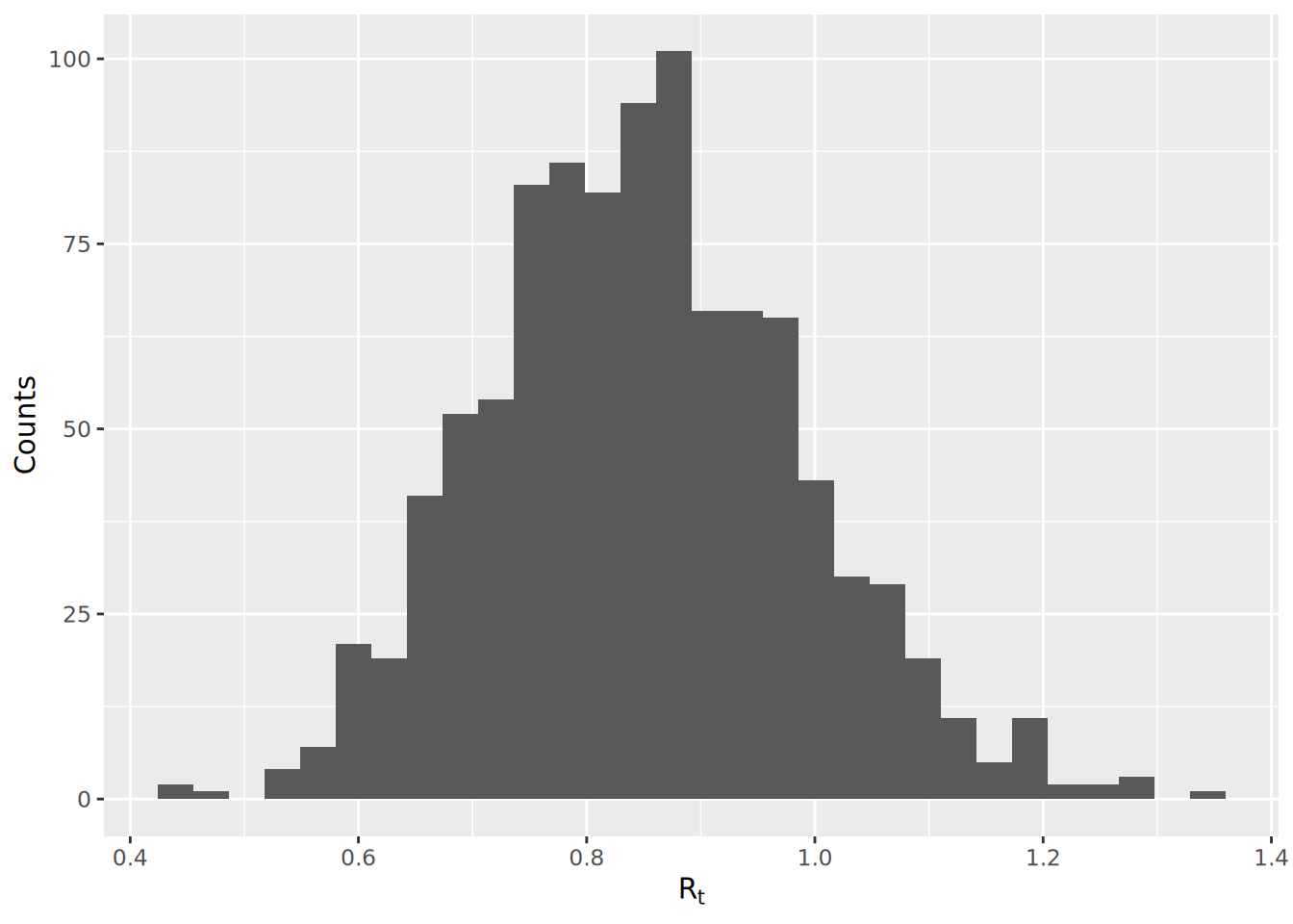
We then use the project() function to make the actual forecast. We specify how many days we want to project for via the n_days arguments, and specify the number of simulations using the n_sim argument.
## make projection
proj <- project(
  x = inc,
  R = plausible_r,
  si = serial_interval$distribution,
  n_days = 21,
  n_sim = 1000
)
We can then plot the incidence with ggplot2 and add the projections with the add_projections() function. The plot() function of incidence raises a deprecation warning from ggplot2, so we do not use it. We can easily subset the incidence object to only show the most recent cases by using the square bracket operator.
## plot the incidence
incidence_plot <- ggplot() +
  geom_col(
    data = as.data.frame(inc[inc$dates > as.Date("2015-03-01")]),
    aes(x = dates, y = counts),
    width = 1
  ) +
  theme_minimal(base_size = 14)

## add the projections
add_projections(incidence_plot, proj)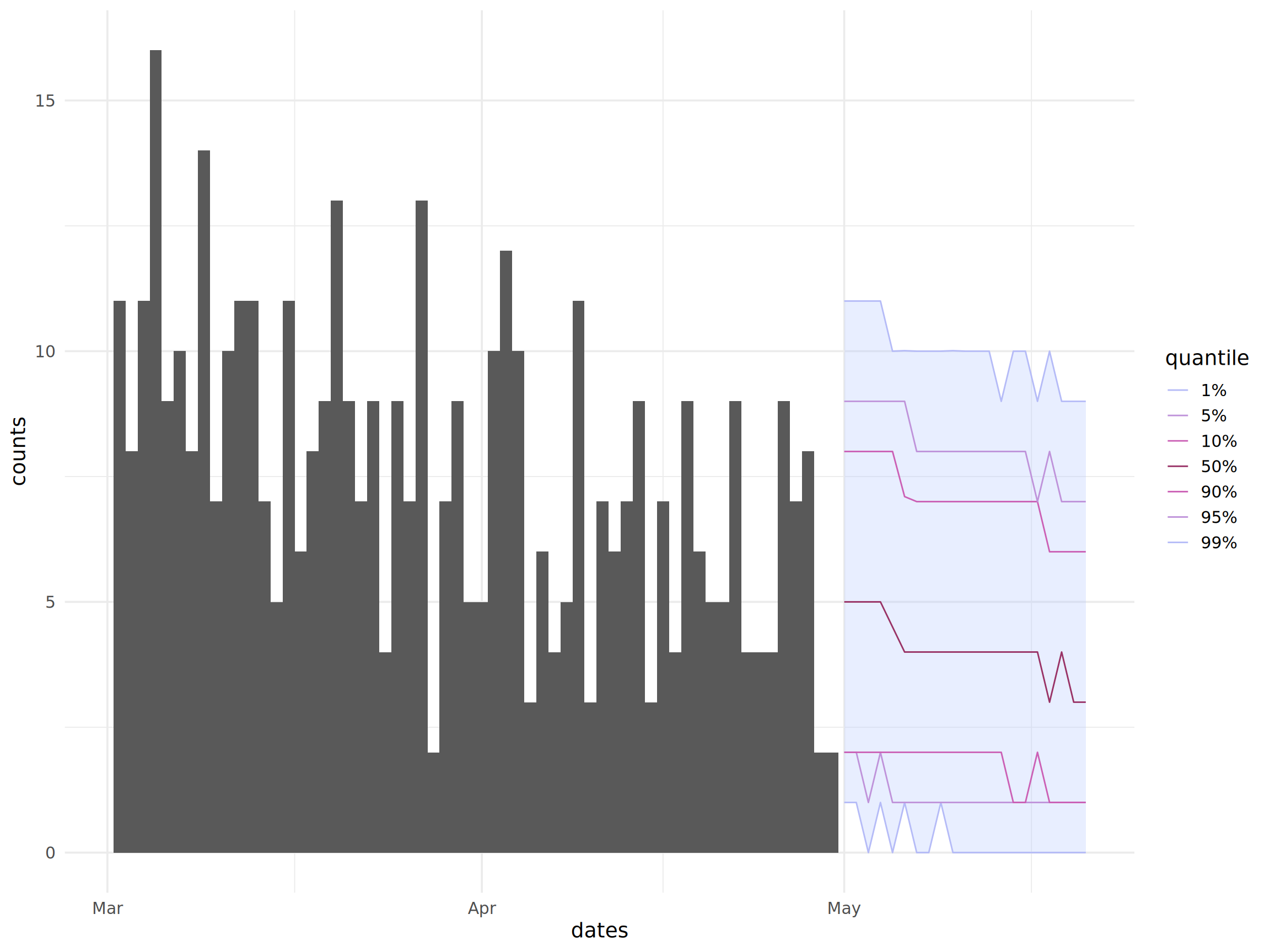
You can also easily extract the raw estimates of daily case numbers by converting the output to a dataframe.
## convert to data frame for raw data
proj_df <- as.data.frame(proj)
proj_df
24.5 Resources
- Here is the paper describing the methodology implemented in EpiEstim.
- Here is the paper describing the methodology implemented in EpiNow2.
- Here is a paper describing various methodological and practical considerations for estimating Rt.